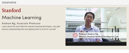
I undertook my first proper online course last year in the shape of Berkeley’s “Introduction to Artificial Intelligence”. Over the last three months I have undertaken and completed a second, Stanford University’s “Machine Learning” taught by Andrew Ng and run by Coursera. It was the same combination that kickstarted the whole Coursera concept four years ago. Machine Learning can broadly be defined as “the study and construction of algorithms that can learn from and make predictions on data“. It’s an important topic in modern computing science closely related to, if not a subset of, Artificial Intelligence and growing in general applicability almost by the day if the tech news agenda is anything to go by:
Machine learning is so pervasive today that you probably use it dozens of times a day without knowing it. Many researchers also think it is the best way to make progress towards human-level AI.
The Stanford course offers a wide-ranging and rigorous introduction to machine learning focussed around three main areas:
- Supervised Learning – fitting a function to data using labeled training samples. Examples covered in the course include: linear regression, logistic regression, support vector machines, neural netwosk
- Unsupervised Learning – fitting a function to describe hidden structure from unlabeled data. Examples covered in the course include: K-means clustering and Principal Component Analysis (PCA)
- Best practice and approaches – including bias vs. variance, working with large datasets and machine learning pipeline construction.
The course doesn’t take in everything there is to cover in Machine Learning. In particular the focus here is on the core disciplines of Supervised and Unsupervised Learning. Reinforcement Learning, which is arguably the third pillar of Machine Learning and of most direct relevance to AI, isn’t covered at all. However, it was examined in some depth in the Berkeley AI material which covered topics like Markov Decision Processes (MDP) and Q Learning.
The core material is presented in a collection of clear and polished video lectures by Professor Andrew Ng who comes across as an engaging and enthusiastic teacher.
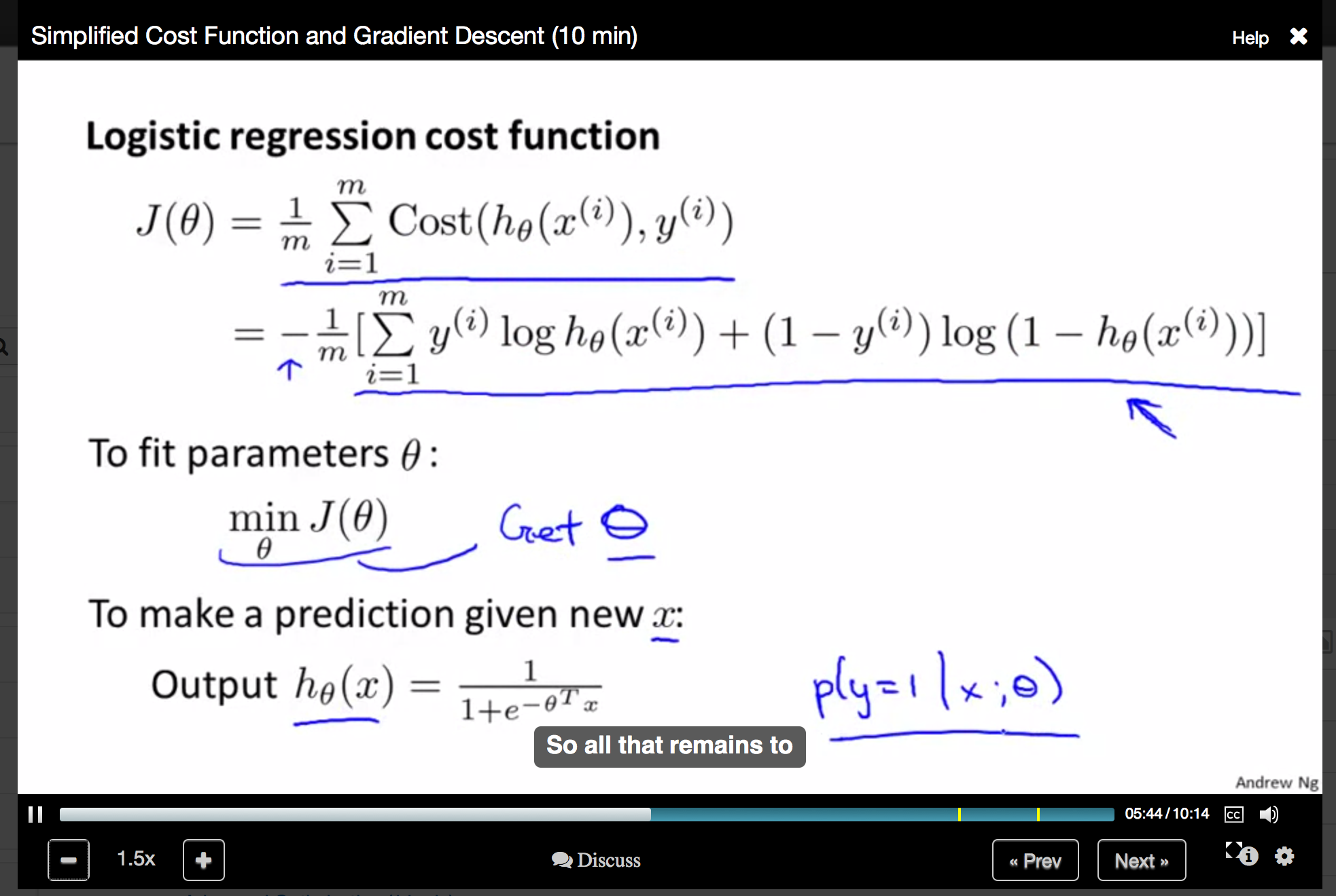
It’s a timed course, with weekly follow-up is in the form of multi-choice quizzes and more demanding working programming exercises which have to be submitted for assessment by an online grader. There’s an interesting identity verification exercise you go through prior to any submission which requires you to type a sentence presumably for comparison of speed with previous submissions. Occasionally you are also obliged to have your photo taken by webcam. The course does a good job of covering a fair amount of machine learning from first principles. Be warned, if you’ve not encountered maths of this variety recently, you may find some of it hard. In this slide, the cost function for logistic regression is being calculated in terms of output prediction based on input x and labelled training output y:
The neural network back propagation algorithm exercise was probably the toughest of the lot and involved a substantial amount of matrix manipulation. If you’re going to undertake the course, it would be advisable to get up to speed on matrix maths especially vectorisation, transposition and the difference between dot product and element-wise matrix multiplication.
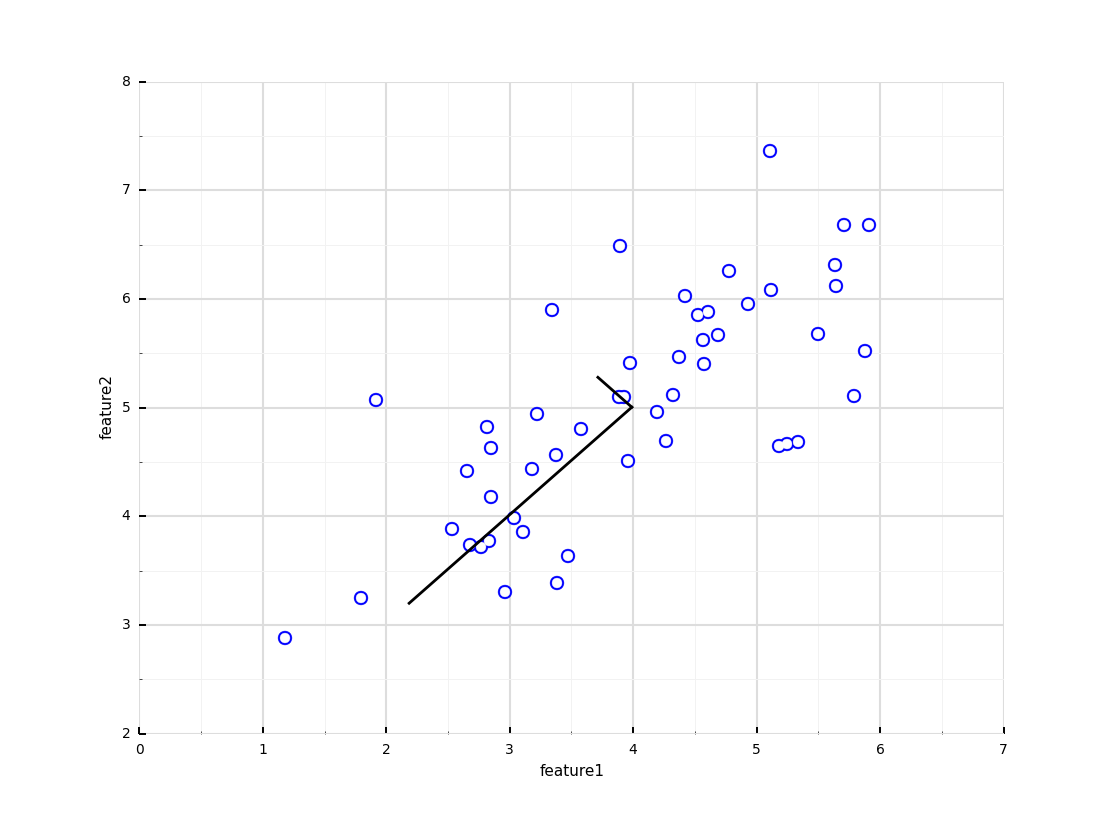
The only real quibble I would raise related to the choice of environment for the programming exercises. MATLAB was chosen because it was considered better for prototyping with but I personally found it a little tricky and idiosyncratic never having worked with it before. MATLAB itself is also non-free though there is a OSS equivalent called Octave. For the course, a free student version of MATLAB that expires after three months or so has been made available. It might have been more approachable to use Python which offers broadly the same level of support used in the exercises through a combination of the powerful numpy, scipy, scikit-learn and matplotlib modules. In fact, since finishing the course, I have been looking to replicate the results of some of the exercises using these Python utilities with a fair degree of success and in many cases substantially less code overall than the MATLAB solution. Below for instance is a fully worked example of PCA, a machine learning technique used to emphasize variation and allow multi-dimensional data to be explored and visualized. The last time I worked with PCA was around 20 years ago when the corresponding implementation required everything from a matrix class in C++ upwards. This solution is built upon the power of numpy operating upon an imported version of the same ex7data1.mat sample data provided in exercise 7 of the course. The code and data are also available on Bitbucket for convenience. Note that the code from Step 3 down isn’t even directly related to the PCA implementation itself – it’s there to convert the data using the pandas module to a form that the ggplot library can display as per the output below:
import numpy as np
import pandas as pd
import scipy.io
from ggplot import *

def loadDataFromMatlabFile(f):
 data = scipy.io.loadmat(f)
 X = data['X']
 return X

def featureNormalize(X):
 # Find average and sigma for numpy matrix columns
 mu = X.mean(0) # columns
 X_norm = X - mu
 sigma = X_norm.std(0,ddof=1)
 X_norm = X_norm / sigma
 return X_norm, mu, sigma

def pca(X):
 m = np.shape(X)[0]
 covarianceMatrix = (1./m) * np.dot(X.T, X)
 return np.linalg.svd(covarianceMatrix)

if __name__ == '__main__':
 # 1. --- Input matrix from Matlab .mat input data file ---
 X = loadDataFromMatlabFile('ex7data1.mat')
 print("Input matrix shape = %s)" % (np.shape(X),))
 assert(np.shape(X) == (50,2))
 # 2. --- Normalize input and run PCA ---
 X_norm, mu, sigma = featureNormalize(X)
 U, S, V = pca(X_norm)
 # 3. --- Convert input to pandas dataframe ---
 f = X.T.tolist()
 assert(len(f) == 2)
 df = pd.DataFrame({'feature1':f[0], 'feature2':f[1]})
 # 4. --- ggplot data overlaid with eigenvectors ---
 # The eigenvectors are centered at mean of data.  Lines
 # show the directions of max variations in the dataset.
 en1 = np.matrix([mu, mu + 1.5 * S[0] * U.T[:,0]])
 en1x,en1y = en1.T[0].tolist()[0], en1.T[1].tolist()[0]
 en2 = np.matrix([mu, mu + 1.5 * S[1] * U.T[:,1]])
 en2x,en2y = en2.T[0].tolist()[0],en2.T[1].tolist()[0]
 plot = ggplot(aes(x='feature1', y='feature2'), data=df) +\
  geom_point(colour='blue',size=100) +\
  geom_point(colour="white", size=50) +\
  geom_line(x=en1x, y=en1y, colour='black', size=2) + \
  geom_line(x=en2x, y=en2y, colour='black', size=2) + \
  theme_seaborn(style='whitegrid')
 print(plot)
Overall the Coursera Machine Learning course was highly enjoyable and a great way to get up to speed on an important discipline of growing relevance to anyone working in a modern tech environment. It constitutes a good base platform on which to take things further. Coursera offer students the chance to pay $32 for a verified course certificate on completion which I’ve now done. I expect to continue using and expanding upon the learning I gained on the course through the coming months and hope to blog some more about it.
31st January 2016